SPH simulation of liquid objects colliding with a surface using PySPH
Full code available on GitHub.
Creating an SPH simulation using PySPH involves defining the particles, equations and the solver. We will simulate how a liquid object falls onto the ground.
Particles
The simulation involves two entities: the object (created from an STL file) and the boundary. We’re going to make them collide. Excited?
STL object
The STL model I chose is a wheel. At first, I didn’t know how to import an STL model into PySPH and use it in the simulation. But then I had an epiphany: I could generate a mesh for the model and place particles in it’s nodes. Genius, isn’t it?
Generating the mesh
First of all, I generated a mesh for the STL model using gmsh.
gmsh.initialize()

path = os.path.dirname(os.path.abspath(__file__))
gmsh.merge(os.path.join(path, 'wheel.stl'))

angle = 40
forceParametrizablePatches = True
includeBoundary = True
curveAngle = 180

gmsh.model.mesh.classifySurfaces(angle * math.pi / 180., includeBoundary,
                                 forceParametrizablePatches,
                                 curveAngle * math.pi / 180.)

gmsh.model.mesh.createGeometry()

s = gmsh.model.getEntities(2)
l = gmsh.model.geo.addSurfaceLoop([s[i][1] for i in range(len(s))])
gmsh.model.geo.addVolume([l])

gmsh.model.geo.synchronize()

f = gmsh.model.mesh.field.add("MathEval")
gmsh.model.mesh.field.setString(f, "F", "4")
gmsh.model.mesh.field.setAsBackgroundMesh(f)

gmsh.model.mesh.generate(3)
gmsh.write('wheel.msh')
Processing the node’s coordinates
The code produces a .msh file, which contains details about the mesh. We are going to open it and extract it’s nodes.
gmsh.initialize()
gmsh.open(path)
nodeTags, nodesCoord, parametricCoord = gmsh.model.mesh.getNodes()
nodesCoord is what we’re interested in. Let’s scale the coordinates (I picked a scale factor so the wheel’s not too big).
scale = 600
x = nodesCoord[0::3]/scale
y = nodesCoord[2::3]/scale
Next, we’ll make our wheel be above the ground by adding the lowest value along the y axis. We additionally raise it to a defined height.
y = y + abs(min(y)) + height
The mesh is dense. I mean 60k nodes dense. We’re going to pick just 6k nodes (every 10th one). Actually, you can try picking more particles. But it would take a while to compute.
x = x[0::10]
y = y[0::10]
Thus, we implemented a function to extract coordinates from an msh file. Creating the particles looks like this.
liquid_x, liquid_y = self.particles_from_model('wheel.msh')
liquid = gpa(name='liquid', x=liquid_x, y=liquid_y)
Walls
Let’s make the walls not too big and not too small: to surround the object, leaving enough room. I decided the room to be 500*dx (500 particles) in each direction.
liquid_x, liquid_y = self.particles_from_model('wheel.msh')

min_x = min(liquid_x) - 500*dx
max_x = max(liquid_x) + 500*dx

min_y = 0
max_y = max(liquid_y) + 500*dx

_x = np.arange(min_x, max_x, dx)
_y = np.arange(min_y, max_y, dx)
x, y = np.meshgrid(_x, _y)
x = x.ravel()
y = y.ravel()
The walls itself are extracted from our overall coordinates array.
walls_x = []
walls_y = []
for i in range(x.size):
    if (y[i] < (min_y + wall_thickness)) or (x[i] >= (max_x - wall_thickness)) or (x[i] <= (min_x + wall_thickness)):
        walls_x.append(x[i])
        walls_y.append(y[i])
Now, we’ve got the arrays of coordinates, where wall particles should be. Let’s generate them.
walls = gpa(name='walls', x=walls_x, y=walls_y)
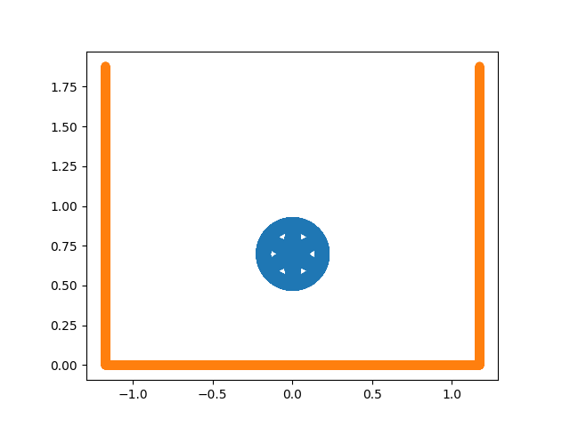
We can preview our setup by plotting it.
plt.scatter(liquid_x, liquid_y)
plt.scatter(walls_x, walls_y)
plt.gca().set_aspect('equal')
plt.show()
Properties
Finally, we define properties for the particles.
# particle volume
liquid.add_property('V')
walls.add_property('V')

# kernel sum term for boundary particles
walls.add_property('wij')

# advection velocities and accelerations
for name in ('auhat', 'avhat', 'awhat'):
    liquid.add_property(name)

liquid.rho[:] = rho0
walls.rho[:] = 5*rho0

liquid.rho0[:] = rho0
walls.rho0[:] = 5*rho0

# mass is set to get the reference density of rho0
volume = dx * dx

# volume is set as dx^2
liquid.V[:] = 1. / volume
walls.V[:] = 1. / volume

liquid.m[:] = volume * rho0
walls.m[:] = volume * rho0

# smoothing lengths
liquid.h[:] = hdx * dx
walls.h[:] = hdx * dx
Equations
The next step is to define the equations, which describe particle’s behavior and boundary conditions. I took them straight out of the hydrostatic_tank example in the PySPH repository (check out other examples, there’s some pretty cool stuff there). I chose the REF3 formulation.
# For the multi-phase formulation, we require an estimate of the
# particle volume. This can be either defined from the particle
# number density or simply as the ratio of mass to density.
Group(equations=[
    VolumeFromMassDensity(dest='liquid', sources=None)
], ),

# Equation of state is typically the Tait EOS with a suitable
# exponent gamma
Group(equations=[
    TaitEOS(
        dest='liquid',
        sources=None,
        rho0=rho0,
        c0=c0,
        gamma=gamma),
    TaitEOS(
        dest='walls',
        sources=None,
        rho0=rho0,
        c0=c0,
        gamma=gamma),
], ),

# Main acceleration block. The boundary conditions are imposed by
# peforming the continuity equation and gradient of pressure
# calculation on the solid phase, taking contributions from the
# fluid phase
Group(equations=[

    # Continuity equation
    ContinuityEquation(dest='liquid', sources=['liquid', 'walls']),
    ContinuityEquation(dest='walls', sources=['liquid']),

    # Pressure gradient with acceleration damping.
    MomentumEquationPressureGradient(
        dest='liquid', sources=['liquid', 'walls'], pb=0.0, gy=gy),

    # artificial viscosity for stability
    MomentumEquationArtificialViscosity(
        dest='liquid', sources=['liquid', 'walls'], alpha=0.25, c0=c0),

    # Position step with XSPH
    XSPHCorrection(dest='liquid', sources=['liquid'], eps=0.5)
])
Solver
Finally, we define the solver.
kernel = CubicSpline(dim=2)
integrator = EPECIntegrator(liquid=WCSPHStep(), walls=WCSPHStep())
solver = Solver(kernel=kernel, dim=2, integrator=integrator,
                tf=tf, dt=dt, adaptive_timestep=True, cfl=0.5, output_at_times=output_at_times)
Running the simulation took about 30 minutes on my PC.
Results
We’ve got some pretty slick results. Check it out!