Multi-label image classification (tagging) using transfer learning with PyTorch and TorchVision
Full code available on GitHub.
Data preprocessing
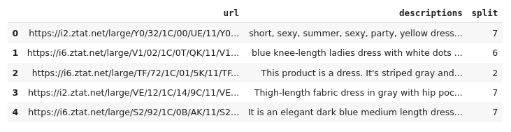
The dataset used is Zalando, consisting of fashion images and descriptions. It’s originally in German, but I translated it with a simple script. You can access the already translated dataset here.
Extracting tags
As you can see, the dataset contains images of clothes items and their descriptions. We are going to extract tags from these descriptions, nouns and adjectives separately. This can be done using ntlk:
def extract_nouns(text):
  tokenized = nltk.word_tokenize(text)
  return [word.lower() for (word, pos) in nltk.pos_tag(tokenized) if pos[:2] == 'NN']

def extract_adjs(text):
  tokenized = nltk.word_tokenize(text)
  return [word.lower() for (word, pos) in nltk.pos_tag(tokenized) if pos[:2] == 'JJ']
Now, that we have a list of nouns and adjectives for every item. The next step is to find the 10 most important ones:
def top_tags(tags):
    counter = TfidfVectorizer(analyzer='word', stop_words='english')
    try:
      counter.fit(tags)
    except ValueError:
      return []

    matrix_count = counter.fit_transform(tags).toarray()
    scores = matrix_count.sum(axis=1)
    sorted_ids = np.argsort(scores).flatten()[::-1]

    return np.array(tags)[sorted_ids[:10]]
To make training faster, we’re going to keep just the 25 most common tags overall (25 nouns and adjs each).
num_classes = 25
all_nouns = df['nouns'].to_numpy()
all_nouns = np.concatenate(all_nouns)
values, counts = np.unique(all_nouns, return_counts=True)
ind = np.argpartition(-counts, kth=num_classes)[:num_classes]
noun_classes = values[ind]
Encoding
Next, we need to convert the tags to vectors (similar to OneHotEncoding, but with multiple tags for each item). The vector will be 50 dimensional as there are 50 tags overall. This is done using MultiLabelBinarizer.
mlb = MultiLabelBinarizer()
y = pd.DataFrame(mlb.fit_transform(df['tags']), columns=mlb.classes_)
Loading the images
In order to make training faster, all the images are loaded beforehand and stored in an array. There are two arrays: one for origin images (pil_images) and one for images, converted to tensors (image_tensors).
image_tensors = []
pil_images = []

img_transforms = transforms.Compose([transforms.Resize((224, 224)), transforms.ToTensor(), transforms.Normalize((0.5, 0.5, 0.5), (0.5, 0.5, 0.5))])

for i, url in enumerate(df['url'].values):
    filename = url.split('/')[-1]
    img = Image.open(f"/content/zalando_img_224/{filename}")
    img = img.convert('RGB')
    pil_images.append(img)
    img_tensor = img_transforms(img)
    image_tensors.append(img_tensor)
When training, it is better to apply some random image transformations to the images to increase validation scores. The transforms are applied to images when they are loaded from the Dataset. All of this logic is implemented in a custom Dataset class:
class MyDataset(Dataset):
    def __init__(self, data, targets):
        self.data = data
        self.targets = torch.Tensor(targets)
        self.transform = transforms.Compose([
                                    transforms.RandomHorizontalFlip(),
                                    transforms.RandomGrayscale(),
                                    transforms.ColorJitter(brightness=0.1, contrast=0.1, saturation=0.1, hue=0.1),
                                    transforms.ToTensor(),
                                    transforms.Normalize((0.5, 0.5, 0.5), (0.5, 0.5, 0.5))
                                ])

    def __getitem__(self, index):
        x = self.transform(self.data[index])
        y = self.targets[index]
        return x, y

    def __len__(self):
        return len(self.data)
Splitting data
Then, the data is split for training and validation.
y = y.to_numpy()

x_train, x_test, y_train, y_test = train_test_split(pil_images, y, test_size=0.3, random_state=42)

train_dataset = MyDataset(x_train, y_train)
dataloader_train = torch.utils.data.DataLoader(train_dataset, batch_size=batch_size, shuffle=True, num_workers=num_workers)

test_dataset = MyDataset(x_test, y_test)
dataloader_test = torch.utils.data.DataLoader(test_dataset, batch_size=batch_size, shuffle=True, num_workers=num_workers)

image_datasets = {'train': x_train, 'val': x_test}
dataloaders = {'train': dataloader_train, 'val': dataloader_test}
Initializing the pretrained Neural Network
We are using the pretrained ResNeXt50 model from PyTorch and modifying the output layer. Also, we’re using a sigmoid function instead of softmax because we treat each label independently.
class Resnext50(nn.Module):
    def __init__(self, n_classes):
        super().__init__()
        resnet = models.resnext50_32x4d(pretrained=True)
        resnet.fc = nn.Sequential(
            nn.Dropout(p=0.2),
            nn.Linear(in_features=resnet.fc.in_features, out_features=n_classes)
        )
        self.base_model = resnet
        self.sigm = nn.Sigmoid()
        self.featureLayer = self.base_model._modules.get('avgpool')

    def forward(self, x):
        return self.sigm(self.base_model(x))

    def getImageVec(self, img):
        image = img.unsqueeze(0).to(device)
        embedding = torch.zeros(1, 2048, 1, 1)
        def copyData(m, i, o): embedding.copy_(o.data)
        h = self.featureLayer.register_forward_hook(copyData)
        model(image)
        h.remove()

        return embedding.numpy()[0, :, 0, 0]

model = Resnext50(num_classes)
model = model.to(device)
model.train()
Finding similar images
Now that we have the model, let’s try finding similar images in our dataset. First, we are going to extract the image’s feature vectors.
image_vectors = []
for image in image_tensors:
    image_vectors.append(model.getImageVec(image))
The cosine distance between two image’s feature vectors indicates how similar they are. Thus, we can find the most similar ones.
random10 = [random.randint(1, len(image_vectors)) for _ in range(10)]

sim_matrix = [];
for i in random10:
    sim_dict = {}
    for j in range(len(image_vectors)):
        sim_dict[j] = cosine_similarity([image_vectors[i]], [image_vectors[j]])[0][0]
    sim_matrix.append(sim_dict)

similar_images = []
for row in sim_matrix:
    sorted_list = sorted(row.items(), key=lambda v: v[1], reverse=True)
    similar = []
    for item in sorted_list[0:5]:
        id = item[0]
        similar.append((df.iloc[id]['url'], item[1]))
    similar_images.append({'id': sorted_list[0][0], 'similar': similar})
Now, let’s see what we’ve got.
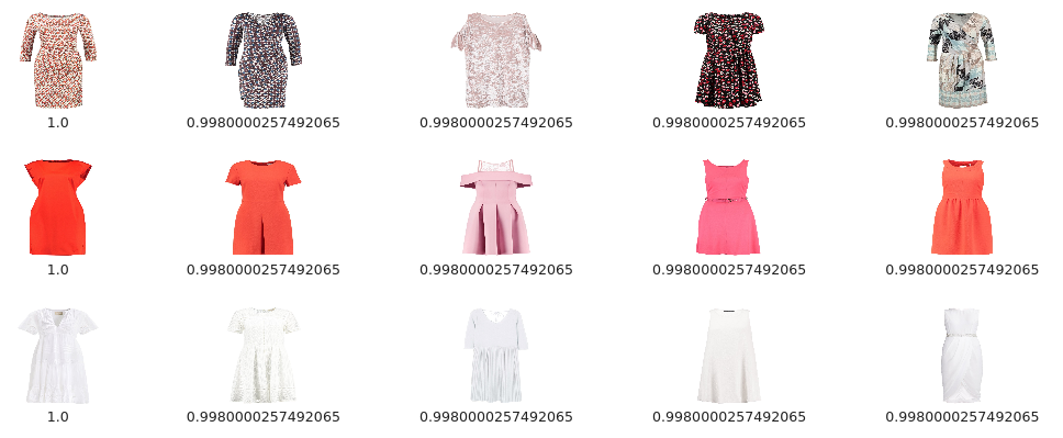
What dress do you like the most in every row? Wait, they’re all similar. Seems legit!
Training
We’re going to use BinaryCrossEntropy loss as it treats all vector components (class) independently.
learning_rate = 1e-3
optimizer = torch.optim.Adam(model.parameters(), lr=learning_rate)
criterion = nn.BCELoss()
Metrics
Calculating f1 score (every 10th iteration).
test_freq = 10

def calculate_metrics(pred, target, threshold=0.5):
    pred = np.array(pred > threshold, dtype=float)
    return {
            'micro/f1': metrics.f1_score(y_true=target, y_pred=pred, average='micro'),
            'macro/f1': metrics.f1_score(y_true=target, y_pred=pred, average='macro'),
            'samples/f1': metrics.f1_score(y_true=target, y_pred=pred, average='samples'),
        }
Saving checkpoints
We’re going to save checkpoints of our model every epoch. Trust me, it’s worth doing.
save_freq = 1
def checkpoint_save(model, epoch):
    f = os.path.join('/content/drive/MyDrive/ml/zalando_checkpoints/', 'checkpoint-{:06d}.pth'.format(epoch))
    if 'module' in dir(model):
        torch.save(model.module.state_dict(), f)
    else:
        torch.save(model.state_dict(), f)
    print('saved checkpoint:', f)
Restoring a checkpoint is simple:
checkpoint = torch.load(os.path.join('/content/drive/MyDrive/ml/zalando_checkpoints/', 'checkpoint-{:06d}.pth'.format(epoch)))
model.load_state_dict(checkpoint)
Now, finally, training!
max_epoch_number = 30

while True:
    batch_losses = []
    for imgs, targets in dataloaders['train']:
        imgs, targets = imgs.to(device), targets.to(device)

        optimizer.zero_grad()

        model_result = model(imgs)
        loss = criterion(model_result, targets.type(torch.float))

        batch_loss_value = loss.item()
        loss.backward()
        optimizer.step()

        batch_losses.append(batch_loss_value)

        if iteration % test_freq == 0:
            model.eval()
            with torch.no_grad():
                model_result = []
                targets = []
                for imgs, batch_targets in dataloaders['train']:
                    imgs = imgs.to(device)
                    model_batch_result = model(imgs)
                    model_result.extend(model_batch_result.cpu().numpy())
                    targets.extend(batch_targets.cpu().numpy())

            result = calculate_metrics(np.array(model_result), np.array(targets))
            print("epoch:{:2d} iter:{:3d} test: "
                  "micro f1: {:.3f} "
                  "macro f1: {:.3f} "
                  "samples f1: {:.3f}".format(epoch, iteration,
                                              result['micro/f1'],
                                              result['macro/f1'],
                                              result['samples/f1']))

            model.train()
        iteration += 1

    loss_value = np.mean(batch_losses)
    print("epoch:{:2d} iter:{:3d} train: loss:{:.3f}".format(epoch, iteration, loss_value))
    if epoch % save_freq == 0:
        checkpoint_save(model, epoch)
    epoch += 1
    if max_epoch_number < epoch:
        break
Training in Google Colab using a GPU took about 2 hours.
Visualising & validating results
Let’s see what we’ve gotby displaying the 3 top tags for each item.
def imshow(inputs):
    img = inputs.transpose(1, 2, 0)
    mean = np.array([0.5, 0.5, 0.5])
    std = np.array([0.5, 0.5, 0.5])
    img = std * img + mean
    inp = np.clip(img, 0, 1)
    plt.imshow(img)

def visualize_model(model, num_images=6):
    model.eval()

    with torch.no_grad():
        for i, (inputs, labels) in enumerate(dataloaders['val']):
            inputs = inputs.to(device)
            labels = labels.to(device)

            outputs = model(inputs)
            preds = outputs.cpu()
            preds = np.array(preds)[0]
            labels = labels.cpu().numpy()

            top3 = np.sort(preds)[::-1][min(2, len(preds)-1)]
            preds[preds < top3] = 0
            preds[preds >= top3] = 1

            tags = mlb.inverse_transform(np.array([preds]))[0][:3]
            tags_real = mlb.inverse_transform(np.array([labels[i]]))[0][:3]

            plt.subplot(2, 3, i + 1)
            plt.axis('off')
            plt.title('Predicted: ' + ', '.join(map(str, tags)) + '\n' + 'Real: ' + ', '.join(tags_real))
            img = np.array(inputs.cpu().data[i])
            imshow(img)

            if i >= num_images - 1:
                return
fig, ax = plt.subplots(figsize=(12,8))
plt.subplots_adjust(hspace=.5, wspace=.5)
visualize_model(model)
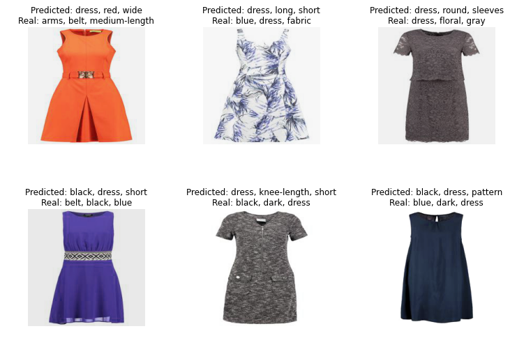
Nice!